<< Back to Blog
August 12, 2025; 15 min read
RNNs Ghosted, LSTMs Goated: The Math Behind It
1. Introduction
When learning long-term dependencies, Recurrent Neural Networks (RNNs) infamously suffer from vanishing and occasionally exploding gradients. Intuitively, as gradients backpropagate through dozens of time steps, they get multiplied by tiny derivatives; it's like playing Telephone, where everyone whispers softer and softer until the message vanishes. It forgets early inputs faster than you forget your online passwords when asked at random.
To address this issue, Hochreiter and Schmidhuber developed the Long Short-Term Memory unit in 1997. For error gradients to loop through time without fading, each LSTM cell has a self-connected node with a fixed weight of 1. This clever technique is known as the Constant Error Carousel, or CEC for short. Furthermore, LSTMs carefully choose what to pass along, what to ignore, and what to keep using input, forget, and output gates.
1.1. The Vanishing and Exploding Gradient Problem in RNNs
1.1.1. Recurrent Computation in Vanilla RNNs
The same transition is carried out repeatedly at each time step as a vanilla RNN processes a sequence.
$$h_t = \phi\bigl(W_h\,h_{t-1} + W_x\,x_t\bigr)$$
- \( W_h \): recurrent weight matrix (same at each time step)
- \( W_x \): input weight matrix
- \( \phi \): activation function (like tanh or sigmoid)
1.1.2. Backpropagation Through Time (BPTT)
Through each time step from \( t+1 \) to \( T \), you apply the chain rule to calculate how the loss \( L \) depends on some earlier hidden state \( h_t \):
$$ \frac{\partial L}{\partial h_t} = \frac{\partial L}{\partial h_T} \cdot \frac{\partial h_T}{\partial h_{T-1}} \cdot \frac{\partial h_{T-1}}{\partial h_{T-2}} \cdots \frac{\partial h_{t+1}}{\partial h_t} $$
\( i.e. \) :
$$ \frac{\partial L}{\partial h_t} = \frac{\partial L}{\partial h_T} \cdot \prod_{k=t+1}^{T} \frac{\partial h_k}{\partial h_{k-1}} $$
Computing \( \frac{\partial h_k}{\partial h_{k-1}} \):
$$h_k = \phi(W_h h_{k-1} + W_x x_k)$$
using chain rule:
$$ \frac{\partial h_k}{\partial h_{k-1}} = \underbrace{\phi'\left( W_h h_{k-1} + W_x x_k \right)}_{\text{diagonal matrix } D_k} \cdot W_h $$
$$ \frac{\partial h_k}{\partial h_{k-1}} = D_k W_h $$
Where \( D_k \) is a diagonal matrix with \( \phi'(\cdot) \) values on the diagonal (\( i.e. \), the derivatives of the activation function). Now, putting everything together, we get :
$$\frac{\partial L}{\partial h_t} \;\propto\; \prod_{k=t+1}^{T} D_k\,W_h $$
when gradients are calculated by backpropagation through \( T \) steps, where \( D_k \) is the diagonal matrix of activation derivatives \( \phi'(\cdot) \) at step \( k \).
If the largest single value of \( D_k W_h \) is on average greater than 1, gradients explode; if it is less than 1, they vanish exponentially over time. In practice, smaller RNNs with sigmoid or tanh activations have issues with vanishing gradients, which makes it difficult to learn from long-term dependencies. Gradient clipping helps with gradients that get too big, but gradients that vanish need changes to the architecture.
2. Long-Short Term Memory (LSTM) Network Architecture
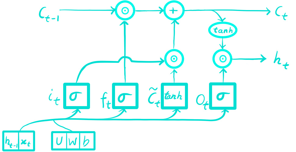
Long Short-Term Memory (LSTM) networks are more advanced than simple RNNs because they have gates and a cell state that control how information flows. During the forward pass, LSTM calculates the input, forget, candidate (cell), and output gates at each time step. It then updates the cell state and hidden state. Let's say the input and the last hidden state. The gate equations are usually written like this (with biases):
$$
\begin{aligned}
i_t &= \sigma(W_i x_t + U_i h_{t-1} + b_i), \\
f_t &= \sigma(W_f x_t + U_f h_{t-1} + b_f), \\
\tilde{c}_t &= \tanh(W_c x_t + U_c h_{t-1} + b_c), \\
c_t &= f_t \odot c_{t-1} + i_t \odot \tilde{c}_t, \\
o_t &= \sigma(W_o x_t + U_o h_{t-1} + b_o), \\
h_t &= o_t \odot \tanh(c_t)
\end{aligned}
$$
:? Feeling lost? Don’t panic, it’ll all make sense soon enough. (smile.png)
Here \(\sigma(\cdot)\) is the sigmoid function, \(\tanh(\cdot)\) is hyperbolic tangent, and \(\odot\) denotes elementwise multiplication.
Notation & Intuition:
\(x_t \in \mathbb{R}^n \Rightarrow\) the input vector at time \(t\) (e.g. a word embedding, an audio feature vector, or a scalar for a single time-series).
\(h_{t-1}\in\mathbb{R}^d \Rightarrow\) the previous hidden state (think of it as the short-term summary the network carries forward).
\(c_{t-1}\in\mathbb{R}^d \Rightarrow\) the previous cell state (this is the LSTM’s long-term memory).
\(i_t,f_t,o_t,\tilde{c}_t,c_t,h_t\in\mathbb{R}^d \Rightarrow\) vectors of length \(d\) (gates and states).
\(W_*\in\mathbb{R}^{d\times n} \Rightarrow\) input-to-gate weight matrices.
\(U_*\in\mathbb{R}^{d\times d} \Rightarrow\) hidden-to-gate (recurrent) weight matrices.
What each gate does?
Input gate \(i_t \Rightarrow\) controls how much of the new candidate \(\tilde c_t\) is written into the cell. (think of it as near 1 meaning write it in, near 0 meaning ignore it.)
Forget gate \(f_t \Rightarrow\) decides how much of the old memory \(c_{t-1}\) is kept. (think of it as near 1 means keeping it, near 0 means erasing it)
Candidate \(\tilde c_t \Rightarrow\) it is the proposed new content (from \(\tanh\)); think of it as raw information, and the input gate \(i_t\) controls how much of it is stored in the cell.
Cell state \(c_t \Rightarrow\) it is the memory belt \(c_t = f_t \odot c_{t-1} + i_t \odot \tilde c_t\) (old kept information plus new written information.)
Output gate \(o_t \Rightarrow\) decides how much of the memory to reveal as the output \(h_t\). (near 1 means show it, near 0 means hide it.)
Together \(W_* x_t + U_* h_{t-1} + b_*\) produces the pre-activation (a \(d\)-vector) for each gate.
Typical dimensions are
$$
x_t\in\mathbb{R}^n,\qquad h_t,c_t\in\mathbb{R}^d,
$$
and therefore
$$
\begin{aligned}
W_i,W_f,W_c,W_o\in\mathbb{R}^{d\times n},\\
U_i,U_f,U_c,U_o\in\mathbb{R}^{d\times d},\\
b_i,b_f,b_c,b_o\in\mathbb{R}^d
\end{aligned}
$$
the gate and state vectors \(i_t,f_t,o_t,\tilde c_t,c_t,h_t\) are all in \(\mathbb{R}^d\), which means that the operations on them are clear. Lastly, you need to set the initial states \(h_0\) and \(c_0\), which are usually set to zero.
Note: You can stack these into a single matrix \(W\in\mathbb{R}^{4d\times (n+d)}\) if you want, but it's usually easier to keep them separate. The forward equations are the same as the standard LSTM formulation; below I give intuition by showing how to compute the transforms via stacking. :)
stacked implementation (efficient form):
$$
\begin{aligned}
W_x &= \begin{bmatrix}W_i\\[4pt]W_f\\[4pt]W_c\\[4pt]W_o\end{bmatrix}\in\mathbb{R}^{4d\times n}, \qquad
W_h = \begin{bmatrix}U_i\\[4pt]U_f\\[4pt]U_c\\[4pt]U_o\end{bmatrix}\in\mathbb{R}^{4d\times d},\\[6pt]
W &= \big[\,W_x \;\; W_h\,\big]\in\mathbb{R}^{4d\times (n+d)}, \qquad
b=\begin{bmatrix}b_i\\[4pt]b_f\\[4pt]b_c\\[4pt]b_o\end{bmatrix}\in\mathbb{R}^{4d}
\end{aligned}
$$
For the concatenated input \(\;\hat{x}_t=\begin{bmatrix}x_t\\[4pt]h_{t-1}\end{bmatrix}\in\mathbb{R}^{n+d}\;\) compute
$$
z_t = W\hat{x}_t + b = \begin{bmatrix}z_{i_t}\\[4pt]z_{f_t}\\[4pt]z_{c_t}\\[4pt]z_{o_t}\end{bmatrix}\in\mathbb{R}^{4d},
$$
and then slice and apply activations:
$$
i_t=\sigma(z_{i_t}); f_t=\sigma(z_{f_t}); \tilde c_t=\tanh(z_{c_t}); o_t=\sigma(z_{o_t})
$$
To keep things simple, I'll keep weight matrices separated in the blog ;)
2.1. Forward Pass
Let's go through forward pass once again carefully so there is no longer any doubt about the shapes or the origins of each vector.
2.1.1. Gated Pre-activations
At each time step the LSTM computes these four intermediate vectors, one for each gate, by linearly combining the current input \(x_t\) and the previous hidden state \(h_{t-1}\) with their corresponding weights and adding biases:
$$
\begin{aligned}
\hat{i}_t &= W_i x_t + U_i h_{t-1} + b_i, \\
\hat{f}_t &= W_f x_t + U_f h_{t-1} + b_f, \\
\hat{\tilde{c}}_t &= W_c x_t + U_c h_{t-1} + b_c, \\
\hat{o}_t &= W_o x_t + U_o h_{t-1} + b_o
\end{aligned}
$$
Here,
\(W_*\) transforms the input into each gate’s computation space (input-to-gate weights).
\(U_*\) transforms the previous hidden state into that same space (hidden-to-gate weights).
\(b_*\) is the bias term that shifts the activation threshold for each gate.
The hats \(\hat{\cdot}\) indicate these are pre-activation values; they are computed before any non-linear function is applied.
(In code you usually compute these four linear combinations in a single matrix multiplication for efficiency; check the stacked version above for reference)
2.1.2. Apply Non-linearities
The actual gate values are obtained by passing the pre-activation values through activation functions: $$ i_t = \sigma(\hat{i}_t); f_t = \sigma(\hat{f}_t); \tilde{c}_t = \tanh(\hat{\tilde{c}}_t); o_t = \sigma(\hat{o}_t) $$ The sigmoid outputs \(i_t, f_t, o_t\) take values in the range \((0,1)\) and control the flow of information/content. The \(\tanh\) output \(\tilde{c}_t\) takes values in \((-1,1)\) and represents the candidate content for the cell state.
2.1.3. Update the Cell State
The new cell state is obtained by combining the previous cell state with the candidate content, weighted by the forget and input gates: $$ c_t = f_t \odot c_{t-1} + i_t \odot \tilde{c}_t, $$ How much of the old memory is kept is determined by the forget gate. The amount of the new candidate that is written into the memory is decided by the input gate.
2.1.4. Compute the Hidden State
The hidden state is obtained by applying the output gate to the activated cell state:
$$
h_t = o_t \odot \tanh(c_t).
$$
How much of the cell's content is exposed to the next layer or next time step is determined by the output gate.
Phew... one step down. The forward pass is just the start. Now, all that remains is to see how gradients flow through time without vanishing. :D
2.2. Backpropagation Through Time \((T)\)
Let's calculate the gradients of a loss \(L\) with respect to all parameters in order to train the LSTM. Gradients are accumulated backward in time by applying the chain rule through the LSTM computational graph. $$ \delta h_t \;=\; \frac{\partial L}{\partial h_t},\qquad \delta c_t \;=\; \frac{\partial L}{\partial c_t} $$ In order to demonstrate how these values are passed back to time step \(t-1\), we will first compute the gradients for each quantity step by step at a single time step \(t\).
2.2.1. Gradients from the Output Gate
From forward pass we have
$$h_t = o_t \odot \tanh(c_t)$$
Derivative of the loss with respect to the output gate vector \(o_t\):
$$\boxed{\;
\delta o_t
\;=\;
\frac{\partial L}{\partial o_t}
\;=\;
\frac{\partial L}{\partial h_t}\odot\frac{\partial h_t}{\partial o_t}
\;=\;
\delta h_t \odot \tanh(c_t)
\;}
$$
contribution to the gradient of the cell \(c_t\) coming from the loss through \(h_t\). By chain rule:
$$
\delta c_t
\;{+}{=}\;
\frac{\partial L}{\partial h_t}\odot\frac{\partial h_t}{\partial c_t}.
$$
(Use \({+}{=}\) to indicate accumulation with any existing \(\delta c_t\).)
compute the Jacobian \(\partial h_t/\partial c_t\) elementwise:
$$
\frac{\partial}{\partial c_t}\big(o_t\odot\tanh(c_t)\big)
\;=\; o_t \odot \big(1-\tanh^2(c_t)\big).
$$
after substituting, we get:
$$\boxed{\;
\delta c_t \;{+}{=} \; \delta h_t \odot o_t \odot \bigl(1-\tanh^2(c_t)\bigr)
\;}$$
2.2.2. Gradients through Cell Update
recall the cell update
$$
c_t = f_t \odot c_{t-1} + i_t \odot \tilde{c}_t,
$$
apply the chain rule:
Derivative w.r.t input gate \(i_t\):
$$\boxed{\;\delta i_t \;=\;\frac{\partial L}{\partial i_t} \;=\; \frac{\partial L}{\partial c_t}\odot\frac{\partial c_t}{\partial i_t}
\;=\; \delta c_t \odot \tilde c_t\;}$$
Derivative w.r.t forget gate \(f_t\):
$$\boxed{\;\delta f_t\;=\;\frac{\partial L}{\partial f_t} \;=\; \delta c_t \odot c_{t-1} \;}$$
Derivative w.r.t candidate \(\tilde c_t\):
$$\boxed{\;\delta \tilde c_t\;=\;\frac{\partial L}{\partial \tilde c_t} \;=\; \delta c_t \odot i_t \;}$$
Contribution back into the previous cell:
$$c_t = f_t \odot c_{t-1} \;+\; ...$$
componentwise: \(c_t[k] = f_t[k]\cdot c_{t-1}[k] + \ldots\).
by the chain rule,
$$
\frac{\partial L}{\partial c_{t-1}[k]}
\;{+}{=}\;
\frac{\partial L}{\partial c_t[k]}\cdot\frac{\partial c_t[k]}{\partial c_{t-1}[k]}
\;=\;
\delta c_t[k]\cdot f_t[k].
$$
stacking components gives the vector form
$$\boxed{\;\delta c_{t-1} += \delta c_t \odot f_t\;}$$
2.2.3. From gate outputs back to pre-activations \((\;\hat.\;)\)
Use activation derivatives componentwise but written as vectors. For sigmoid \(\sigma(z)\) ; \(\sigma'(z)=\sigma(z)(1-\sigma(z))\): $$\boxed{\; \begin{aligned} \frac{\partial L}{\partial \hat i_t} = \frac{\partial L}{\partial i_t}\odot i_t\odot(1-i_t);\\[7pt] \frac{\partial L}{\partial \hat f_t} = \frac{\partial L}{\partial f_t}\odot f_t\odot(1-f_t);\\[7pt] \frac{\partial L}{\partial \hat o_t} = \frac{\partial L}{\partial o_t}\odot o_t\odot(1-o_t) \end{aligned}\;}$$ for the candidate \(\tilde c_t=\tanh(\hat{\tilde c}_t)\): $$ \boxed{\; \frac{\partial L}{\partial \hat{\tilde c}_t} = \frac{\partial L}{\partial \tilde c_t}\odot\bigl(1-\tilde c_t^2\bigr) \;} $$ for ease, you can name these pre-activation gradients \(\delta\hat i_t,\delta\hat f_t,\delta\hat o_t,\delta\hat{\tilde c}_t\).
2.2.4. Parameter gradients
recall \(\hat v_t = W_v x_t + U_v h_{t-1} + b_v\) for \(v\in\{i,f,o,c\}\). per time-step contributions (then sum over \(t\) to get full gradients): input weights: $$ \frac{\partial L}{\partial W_v} \;{+}{=}\; \delta\hat v_t\, x_t^\top $$ (don't get confused; over here \(\delta\hat v_t\, x_t^\top\) is the outer product of the pre-activation gradient with the input.) now hidden weights: $$ \frac{\partial L}{\partial U_v} \;{+}{=}\; \delta\hat v_t\, h_{t-1}^\top $$ and finally bias: $$ \frac{\partial L}{\partial b_v} \;{+}{=}\; \delta\hat v_t $$
2.2.5. Backprop into \(h_{t-1}\) and \(x_t\)
each gate pre-activation \(\hat v_t\) is linear in \(h_{t-1}\) and \(x_t\), so the loss gradient flowing into \(\hat v_t\) is routed back into \(h_{t-1}\) and \(x_t\) via the corresponding weight matrices
to previous hidden state \((\;h_{t-1}\;)\):
$$
\frac{\partial L}{\partial h_{t-1}} \;{+}{=}\;
U_i^\top \delta\hat i_t \;+\; U_f^\top \delta\hat f_t \;+\; U_c^\top \delta\hat{\tilde c}_t \;+\; U_o^\top \delta\hat o_t
$$
to input \((x_t)\):
$$
\frac{\partial L}{\partial x_t} \;{+}{=}\;
W_i^\top \delta\hat i_t \;+\; W_f^\top \delta\hat f_t \;+\; W_c^\top \delta\hat{\tilde c}_t \;+\; W_o^\top \delta\hat o_t
$$
(here, you can see that these are just the sum of each gate’s pre-activation gradient multiplied by the corresponding weight transpose.)
2.2.6. Time recursion and backward algorithm
For \(t=T,T-1,\dots,1\) do:
1. Start with \(\delta h_t\) (from the loss or future time steps / upper layers).
2. Compute output pre-gate gradient:
$$
\delta o_t \;=\; \delta h_t \odot \tanh(c_t)
$$3. Add hidden \(\rightarrow\) cell contribution:
$$
\delta c_t \;{+}{=}\; \delta h_t \odot o_t \odot \bigl(1-\tanh^2(c_t)\bigr)
$$4. From the cell update compute:
$$
\begin{aligned}
\delta i_t \;=\; \delta c_t \odot \tilde c_t,\\
\delta f_t \;=\; \delta c_t \odot c_{t-1},\\
\delta \tilde c_t \;=\; \delta c_t \odot i_t
\end{aligned}$$5. Push through activation derivatives to get \(\delta\;\hat{\cdot}_t\) as in 2.2.3.
6. Accumulate parameter gradients \(\partial L/\partial W_v,\ \partial L/\partial U_v,\ \partial L/\partial b_v\) as in 2.2.4.
7. Accumulate \(\partial L/\partial h_{t-1}\) and \(\partial L/\partial x_t\) as in 2.2.5.
8. Propagate cell gradient back in time:
$$
\delta c_{t-1} \;{+}{=} \; \delta c_t \odot f_t
$$9. Move to \(t-1\).
2.2.7. Gradient flow intuition
The backward recurrence
$$
\delta c_{t-1} = \delta c_t \odot f_t
$$
shows why LSTMs resist vanishing gradients; propagating this relation backwards for \(k\) steps gives:
$$
\frac{\partial L}{\partial c_{t-k}} = \frac{\partial L}{\partial c_t} \odot \prod_{j=t-k+1}^{t} f_j
$$
If each forget-gate output \(f_j\) is near 1 (per component), the product remains close to 1, allowing gradients to pass unchanged across long spans. If the \(f_j\) values are small, the product shrinks and gradients fade.
The self-connection \(c_{t-1} \to c_t\) was fixed in the original LSTM design, ensuring that \(\partial c_t / \partial c_{t-1} = 1\) whenever the gates were open. Learnable forget gates are used in place of this in modern LSTMs, allowing the model to dynamically determine when to overwrite and when to preserve information.
3. LSTM implementation and intuition
Hah... finally, done with the math. Now, let's implement an LSTM in Python using NumPy. Lessgoo! :)
import numpy as np
def sigmoid(x):
    return 1 / (1 + np.exp(-x))
def dsigmoid(x):
    return x * (1 - x)
def tanh(x):
    return np.tanh(x)
def dtanh(x):
    return 1 - np.tanh(x) ** 2
def softmax(x):
    e_x = np.exp(x - np.max(x))
    return e_x / e_x.sum(axis=0, keepdims=True)
def dsoftmax(x):
    s = softmax(x)
    return s * (1 - s)

class LSTM:
    def __init__(self, input_size, hidden_size, num_layers=1, forget_bias=1.0, seed=None):
        if seed is not None:
            np.random.seed(seed)
        self.n = input_size
        self.d = hidden_size
        self.L = num_layers
        self.params = []
        for layers in range(self.L):
            in_dim = self.n if layers == 0 else self.d
            scale = 1.0 / np.sqrt(in_dim)
            W = np.random.randn(4 * self.d, in_dim) * scale
            b = np.zeros(4 * self.d)
            b[self.d:2 * self.d] = forget_bias
            self.params.append({
                'W': W,
                'b': b
            })
        self.last_cache = None
    def forward(self, x, h_prev=None, c_prev=None):
        if h_prev is None:
            h_prev = np.zeros((self.L, self.d))
        if c_prev is None:
            c_prev = np.zeros((self.L, self.d))
        h = []
        c = []
        cache = []
        for layers in range(self.L):
            W, b = self.params[layers]['W'], self.params[layers]['b']
            z = np.dot(W, x) + b
            i = sigmoid(z[:self.d]) # input gate
            f = sigmoid(z[self.d:2 * self.d]) # forget gate
            o = sigmoid(z[2 * self.d:3 * self.d]) # output gate
            g = tanh(z[3 * self.d:]) # candidate cell gate
            c_new = f * c_prev[layers] + i * g # new cell state
            h_new = o * tanh(c_new) # new hidden state
            h.append(h_new)
            c.append(c_new)
            cache.append({'z': z, 'i': i, 'f': f, 'o': o, 'g': g, 'x': x.copy(), 'c_prev': c_prev[layers].copy(), 'c_new': c_new.copy(), 'W': W})
            x = h_new
        self.last_cache = cache
        return np.array(h), np.array(c)
    def backward(self, dh, dc, h_prev, c_prev):
        dW = []
        db = []
        for layers in reversed(range(self.L)):
            W, b = self.params[layers]['W'], self.params[layers]['b']
            h_new = h_prev[layers]
            c_new = c_prev[layers]
            cache = self.last_cache[layers] if self.last_cache is not None else {}
            z = cache.get('z', np.zeros(4 * self.d))
            i = cache.get('i', np.zeros(self.d))
            f = cache.get('f', np.zeros(self.d))
            o = cache.get('o', np.zeros(self.d))
            g = cache.get('g', np.zeros(self.d))
            x = cache.get('x', np.zeros(z.shape[0] // 4 if z.shape[0] else 1))
            do = dh * tanh(c_new) # gradient w.r.t. output gate
            dc_new = dc + dh * o * dtanh(c_new) # gradient w.r.t. cell state
            di = dc_new * g # gradient w.r.t. input gate
            df = dc_new * c_prev[layers - 1] if layers > 0 else np.zeros_like(dc_new) # gradient w.r.t. forget gate
            dg = dc_new * i # gradient w.r.t. candidate cell gate
            dz = np.zeros_like(z)
            dz[:self.d] = di * dsigmoid(i)
            dz[self.d:2 * self.d] = df * dsigmoid(f)
            dz[2 * self.d:3 * self.d] = do * dsigmoid(o)
            dz[3 * self.d:] = dg * (1 - g * g)
            dW.append(np.outer(dz, x))
            db.append(dz)
            dh = np.dot(W.T, dz)
        dW.reverse()
        db.reverse()
        return dW, db
    def update_params(self, dW, db, learning_rate=0.01):
        for layers in range(self.L):
            self.params[layers]['W'] -= learning_rate * dW[layers]
            self.params[layers]['b'] -= learning_rate * db[layers]
    def train(self, x, y, epochs=100, learning_rate=0.01):
        for epoch in range(epochs):
            h_prev, c_prev = None, None
            loss = 0
            for t in range(len(x)):
                h, c = self.forward(x[t], h_prev, c_prev)
                h_prev, c_prev = h[-1], c[-1]
                loss += np.mean((h[-1] - y[t]) ** 2)
                dh = h[-1] - y[t]
                dc = np.zeros_like(c[-1])
                dW, db = self.backward(dh, dc, h, c)
                self.update_params(dW, db, learning_rate)
            print(f'Epoch {epoch + 1}/{epochs}, Loss: {loss / len(x)}')
    def predict(self, x):
        h_prev, c_prev = None, None
        for t in range(len(x)):
            h, c = self.forward(x[t], h_prev, c_prev)
            h_prev, c_prev = h[-1], c[-1]
        return h[-1]
    def reset_state(self):
        self.h_prev = np.zeros((self.L, self.d))
        self.c_prev = np.zeros((self.L, self.d))

if __name__ == "__main__":
    input_size = 10
    hidden_size = 20
    lstm = LSTM(input_size, hidden_size, num_layers=2, seed=42)
    x = np.random.randn(5, input_size)
    y = np.random.randn(5, hidden_size)
    lstm.train(x, y, epochs=10, learning_rate=0.01)
    prediction = lstm.predict(x)
    print("Prediction:", prediction)
Thanks for reading till the end, you absolute legend being!
You have backpropagated through all the paragraphs. (•̀ᴗ•́)و
Until next time, happy learning!